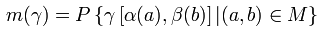
If you are searching for resources to help you understand how one can go about linking records “probabilistically”, you will find many resources that all pretty much start the same way, “probabilistic record linkage…[yadda, yadda]…theory formalized by Fellegi and Sunter (1969)…”, and then quickly move to a discussion of matching vectors and the calculation of m and u probabilities using formulas like:

This approach unnecessarily obfuscates a relatively simple concept (although it does a wonderful job of protecting an academic discipline and tenure…). I will attempt here to introduce the general approach to probabilistic record matching while keeping obfuscation to a minimum.

General Approach

The general approach to probabilistic record linkage is fairly straight-forward. To figure out if two records from two different data sets match, matching record fields from the two data sets are compared (e.g. a field that records “Last Name” that is in both data sets). To determine if matching fields are “better” or “worse” for using in this matching process, we need to know two things: how reliable is the data in those fields, and how common are the values in those fields? That’s it.

If a field is not reliably collected, it loses its ability to help with record matching. For example, if we know from past experience that in a particular data set the field “Birthdate” is only about 50% reliable (because of a combination of non-entries, guessing, and a dyslexic data clerk), then we know “Birthdate” won’t be helping us with our matching at all. Flipping a coin would give you the same results.

If a field value is too common, it also loses its ability to help with record matching. For example, if we are looking at two data sets from New York City, and all of the records in both data sets list “New York City” in the address field “City”, then we know that the field “City” is also useless for the purpose of record matching. It doesn’t help winnow down the likely matches at all.

Now, if we are looking at two data sets for which data has been meticulously collected, and the commonness of field values is sufficiently varied, we have a much better chance of finding a true match between two data records. For example, if we have two very well maintained data sets that each have only one record with a value of “McGillicuddy” for the field “Last Name” and “Barrow, Alaska” for the fields “City” and “State”, then we have a very high probability that these records do in fact match.

The problem of course is that while a knowledgeable person can make data set by data set, and record by record value judgments to decide whether to link records or not, that person can’t efficiently go through millions of possible combinations in any sort of timely fashion (e.g. if file A contains 1,000 records, and file B contains 10,000 records, the number of possible record pairs is 1,000 x 10,000, 10 million record pairs).

So, we are left needing to get a computer program to adequately determine the likelihood of two records matching based on the reliability and commonness of the data field values given. This is the problem that Fellegi and Sunter set out to address. They did such a good job that their model is at the base of just about every matching software on the market today. Improvements in the field have mostly taken the form of improving the inputs to their original model.

The Model Basics

In the Fellegi and Sunter probabilistic model, two fields are compared and a measure is assigned reflecting how similar the field values are. This measure is referred to as the “field weight” and it is calculated based on the reliability of the data in the matching field and the commonness of values in the matching field.

The reliability of the data is represented by what is called the “m probability”, and the commonness of the value is represented by what is called the “u probability” (more on these below). Once we have our “m” and “u” probabilities, we can calculate “field weights” for when two values “agree” or “disagree”. The weights for agree/disagree are (usually) different. \ For example, if Gender is meticulously collected and the values for two records for Gender do not match, that gives us pretty strong evidence that the records don’t match. So, “disagreement” on Gender would be heavily weighted. However, if Gender is meticulously collected and the values for two records for Gender \textbf{do} match, that \textbf{does not} give us very strong evidence that the two records actually match (it only narrows the field of possible matches by approximately 50\%). Therefore, “greement” on Gender gets weighted much less than “disagreement”.

Once we have our agree/disagree field weights, then, for each comparison pair, the weights for each compared field are simply summed up into a “composite weight”. While it is certainly a simplification, at this point the important bit to understand is that positive composite weights represent “matches” and negative composite weights represent “non-matches”.

An example

Let’s start with two data sets, A and B. For each data set we have the fields Name, Gender (Gen), and Date of Birth (DOB).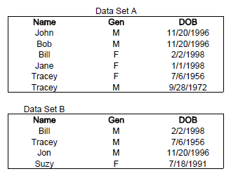

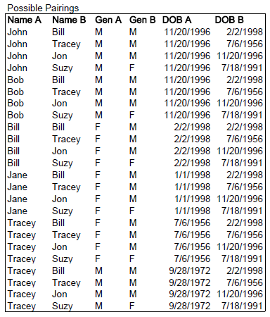
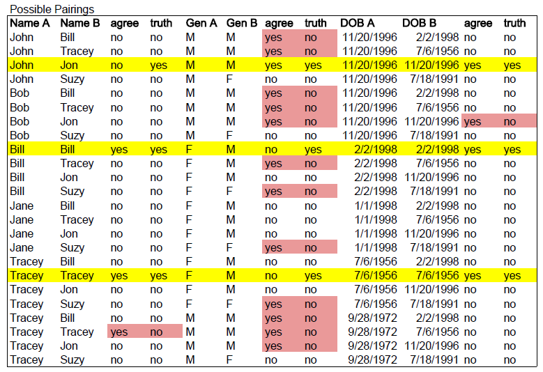
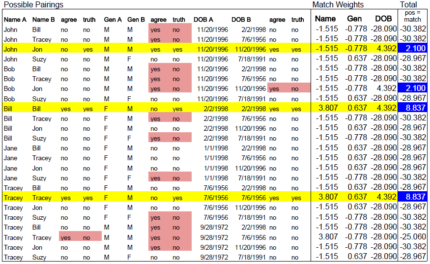
As discussed, we will first need to figure out the reliability and commonness of the field value pairs we are dealing with. To start, let’s list all of the possible pairings from these two data sets. 6 records in Data Set A multiplied by 4 records in Data Set B gives us 24 possible pairings.

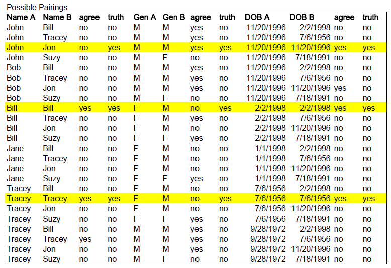
Now let’s add two columns for each field pairing. The first column we will name “agree” and it will take the values “yes” or “no” if the two values are the same. The second column we will name “truth” and it will take the values “yes” or “no” representing whether or not the two records actually match (we might know this from previous history, a shared identifier like SSN, or a manual processing of a sample of records for just this purpose). \ In the figure below, the highlighted record pairings represent records that we know match. If we look at the first highlighted pairing, we can see that while the names “John” and “Jon” do not agree, the records do in fact match (hmmm, looks like there might some quality problems with name input for one of these sets).

The m and u probabilities

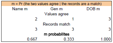
With this data, we now have all we need to figure out our m and u probabilities.

The m probability (quality) can be expressed as the probability that two field values agree given that that the two records they come from are in fact a match. That is, if we have two records that we know match, then all of the paired field values should, in a perfect world, match. If some of the fields don’t match, then we have some degree of quality/reliability problem with those fields.

So, looking at the table, how many records do we know that match? Three. OK, then, just looking at those three record matches, how many times do the values agree for each field pair? For example, looking at the pairing of Name A and Name B, we see that 2 out of 3 times the values agree. Therefore, the m probability for Name is 2/3 or 0.667. The results are summarized below.

The u probability (commonness) can be expressed as the probability that the two field values agree given that the records they came from are in fact \textbf{not} a match. Or, the other way around, if we have two records that we know don’t match, how likely is it that the values in a particular field pairing (e.g. “City”) will match anyway (because of the relative commonness of the values)?

Looking at the table again, we want to determine how many times the value agrees in a pairing when the records do not in fact match. These are highlighted in red. Just looking at the red, it is easy to quickly pick up on the fact that there are many times when the values for Gender agree, but the records do not actually match. So, just from visual inspection alone, we can determine that Gender is not a very good for determining a match between records (many more that agree are not actually matches!).

The calculations for the u probability for each field pair are presented here.

Field Weights

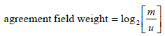
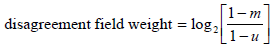
Once we have m and u, we can now calculate the weights for each field pair. Which calculation to use depends on whether or not the two values in the field agree. If they do agree, a positive weight is generated, and if they disagree a negative weight is generated. The size of the weight measures the evidence the values provide about the record pair being a match. The two calculations are:

So, for the m and u probabilities we found, our weights are:

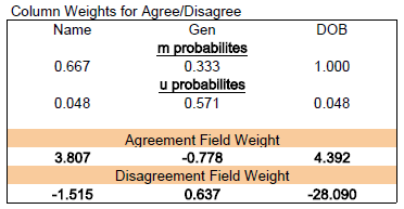
Looking at the results for “Name”, we see that if a field pair agrees, it gets assigned a 3.807, but if it disagrees, it gets assigned a -1.515.

You may have also noticed that in the Column Weights calculations above that the agree weight for “Gen” is negative and the disagree weight is positive. This is of course inconsistent with what I stated about the agree formula giving a positive number and the disagree giving a negative number. In practice this doesn’t happen, but it is good for illustration here. Because we are only looking at three matched records in this example, the fact that 2 out of the 3 field pairing for Gender don’t agree has the effect of actually making an agreement on Gender negative. After all, if you found agreement on Gender in this particular data set, you’d actually be wrong 2/3 of the time! As I stated, this isn’t what happens in practice, but it does illustrate the effect of unreliable data.

The Composite Weight - Add it all up

Now that we have our agree/disagree weights for each field pair, we can go ahead and assign the weights and then calculate the total composite weight for each record pairing. In the table below, the cells in the Total column that are highlighted blue indicate the composite scores that indicate a match (they are positive). Our probabilistic matching process successfully found the matches we knew to be true!

However, it also identified one match where a match does not in fact exist (between Bob and Jon). What happened?

Well, if we go back and look at the m probability calculated for DOB, we find that it is a perfect 1. That is, the reliability of that field is 100%! This doesn’t actually occur in practice, but it illustrates how powerful reliable data can be (it gets both the highest weight for agreement and lowest for disagreement). And, because we only have three fields we are looking at, and one of them is very unreliable (Gender), DOB has a lot of power to influence the composite score. In fact, if we look at the pairing of the male and female Traceys, we can see that even though there was agreement on two of the three fields (Name and Gender), just like with Bob and Jon, they were correctly identified as not being a match (because the weights for those two are not as important as DOB which, in this example, is 100\% reliable).

Finding m and u probabilities in practice

m

In practice, figuring out data quality (e.g. error rates in data entry) can be difficult. The best method, sampling with manual comparison, is also the most labor intensive. Sometimes, especially when dealing with a-typical type data sets, it is necessary. Generally, however, one of two approaches will suffice.

When very large data sets are being used, and each employs some form of highly reliable unique identifier (e.g. SSN in one, STI in another), then each set can be “self-joined” on that identifier and discrepancies in field values for the same individual identified. For example, using the Virginia Student Record data set, we can “self-join” on STI and then look for how many times Gender doesn’t match even though STI does match. This discrepancy rate would give us a quality measure for the field Gender for that data set. If then matched against another large data set on Gender, the m probability can be calculated as the product of the two discrepancy rates found.

The method most commonly employed to determine m probabilities is simply heuristic. Record linkage practitioners have found over the years that field reliability is determined, for the most part, by the relative importance of the field for supporting the core operational requirements of the agency using the data set. For example, the address field is a very important field to an agency like the IRS that has to mail refund checks (and find tax evaders!). A common rubric employed for assigning m probabilities is:

Very important fields: 0.999 Moderately important fields: 0.95 Most fields: 0.9 Poor reliability fields: 0.8

Running a self-join on over 2 million records from the Virginia Student Record, and making some assumptions about which fields get which level of importance, I found numbers very similar to the suggested rubric.

A great deal of the literature on probabilistic record matching concerns newer and more mathematically fancy methods of estimating m probabilities. While improvements are certainly being found, in practice, none has surpassed the accuracy of running a basic probabilistic model followed by human review of the “borderline” cases.

u

The example given here illustrates what u probabilities are and how they are determined. It does not accurately illustrate how they are actually employed in some cases. For a field like DOB that has a close-to-uniform distribution, the u probability is generally calculated on the whole field (as is done here). \ For fields that do not have a uniform distribution, such as Last Name, u probabilities are generally determined for each value of that field. For example, “McGillicuddy” will have a much lower u probability than “Smith”, therefore, we want to calculate and run them separately.