Introduction to floating catchment areas
Floating catchment area (FCA) methods measure how much supply (clinics, jobs,
services) is accessible to each unit of demand (population), accounting for
the travel cost between them. catchment_ratio is the single entry point: you
give it consumer and provider tables, a travel-cost matrix, and a rule for how
cost turns into a weight — a hard distance bound, a decay kernel, or both. Every
FCA variant (2SFCA, E2SFCA, gravity, …) is a choice of those parameters.
Setup
A tiny catchment
Three equally-populated consumers sit in a line; two equal-capacity providers sit at the ends. We build the travel-cost matrix from coordinates, then compute access two ways.
# 3 consumers (demand, value = population), 2 providers (supply, value = capacity).
consumers = pd.DataFrame({"geoid": ["c1", "c2", "c3"], "value": [100.0, 100.0, 100.0]})
providers = pd.DataFrame({"geoid": ["p1", "p2"], "value": [10.0, 10.0]})
consumers_xy = np.array([[0.0, 0.0], [1.0, 0.0], [2.0, 0.0]])
providers_xy = np.array([[0.0, 0.0], [2.0, 0.0]])
cost = euclidean_cost(consumers_xy, providers_xy)

# Binary catchment: everyone within max_cost=3.0 counts equally.
binary = catchment_ratio(consumers, providers, cost, max_cost=3.0)
# Distance-decay catchment: gaussian kernel.
decay = catchment_ratio(consumers, providers, cost, weight="gaussian", scale=1.0)

print("cost matrix:\n", cost)
print("\nbinary access:\n", binary.to_string())
print("\ngaussian-decay access:\n", decay.to_string())
cost matrix:
 [[0. 2.]
 [1. 1.]
 [2. 0.]]

binary access:
 c1    0.066667
c2    0.066667
c3    0.066667

gaussian-decay access:
 c1    0.065179
c2    0.069641
c3    0.065179
With a generous binary bound, every consumer reaches both providers and receives
the region-wide supply-to-demand ratio — total supply 20 over total demand 300,
or about 0.0667 units of capacity per person. Switching to a gaussian decay
differentiates by distance: the central consumer c2, closest on average to both
providers, gets the highest access, and the two ends get slightly less.
Decay behaviour is set by the weight kernel and its scale. KERNELS provides
linear, gaussian, gravity, exponential, logistic, and logarithmic;
max_cost adds a hard travel bound on top of any kernel.
On real geography
The same call scales straight to real data. Here every block group in Arlington
County, VA is a demand unit (located at its centroid), with three clinics placed
inside the county. The block-group geometries ship with this page as
county_bgs.geojson; we project to UTM 18N so distances are in meters.
import numpy as np
import pandas as pd
import geopandas as gpd
from sdc_catchment import catchment_ratio, euclidean_cost

# Arlington County's 204 block groups (ships with this page), projected to meters.
bgs = gpd.read_file("county_bgs.geojson").to_crs(32618).reset_index(drop=True)
bgs["geoid"] = bgs["geoid"].astype(str)
cent = bgs.geometry.centroid
bg_xy = np.c_[cent.x.values, cent.y.values]

# Each block group is a demand unit with a synthetic population.
rng = np.random.default_rng(0)
consumers = pd.DataFrame({"geoid": bgs["geoid"], "value": rng.integers(500, 2500, len(bgs)).astype(float)})

# Three clinics inside the county (centroids of 3 evenly-spaced block groups).
idx = np.linspace(0, len(bgs) - 1, 3).astype(int)
clinics = pd.DataFrame({"geoid": ["A", "B", "C"], "value": [20.0, 15.0, 30.0]})
cost = euclidean_cost(bg_xy, bg_xy[idx])

access = catchment_ratio(consumers, clinics, cost, weight="gaussian", scale=2000.0, max_cost=8000.0)
beds_per_1000 = (access * 1000).round(3)
print(beds_per_1000.head().to_string())
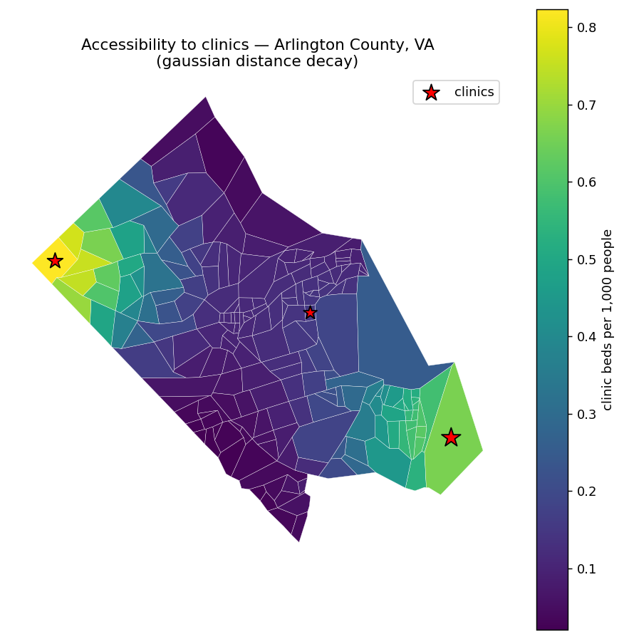
Each block group is shaded by clinic beds accessible per 1,000 residents; access
falls off with distance from the three clinics (stars). This is the same
catchment_ratio call as above, on 204 real block groups instead of three points.