7 A Second Approach: Parcel-Based Redistribution
The area-weighted method introduced in Chapter 4 works well, but it rests on a simplifying assumption worth examining: that each variable of interest is distributed uniformly across a block group’s entire polygon. In practice, a block group’s polygon includes roads, parks, parking lots, commercial strips, and other land that contains no housing at all. For measures tied to where people actually live, this matters. Dasymetric methods replace the uniform-distribution assumption by using an ancillary layer (in this case, parcel locations) to concentrate redistributed values where housing actually sits [1].
This chapter implements that alternative and then asks directly: how much does the choice of method change the result?
7.1 The parcel data
Arlington County’s Master Housing Unit Database (MHUD) provides a parcel-level inventory of every residential unit in the county. The layer used here contains 34,340 parcels carrying roughly 127,000 housing units in total. The vast majority of those parcels (33,665) are single-family detached or attached (SFD/SFA) structures, typically carrying one or two units apiece. The remaining 675 parcels are classified as multifamily (MULTI), and they account for a disproportionate share of the county’s housing stock: the multifamily parcels are concentrated along the Rosslyn–Ballston corridor and the Route 1 spine, where high-rise and mid-rise buildings each contribute hundreds of units to the total.
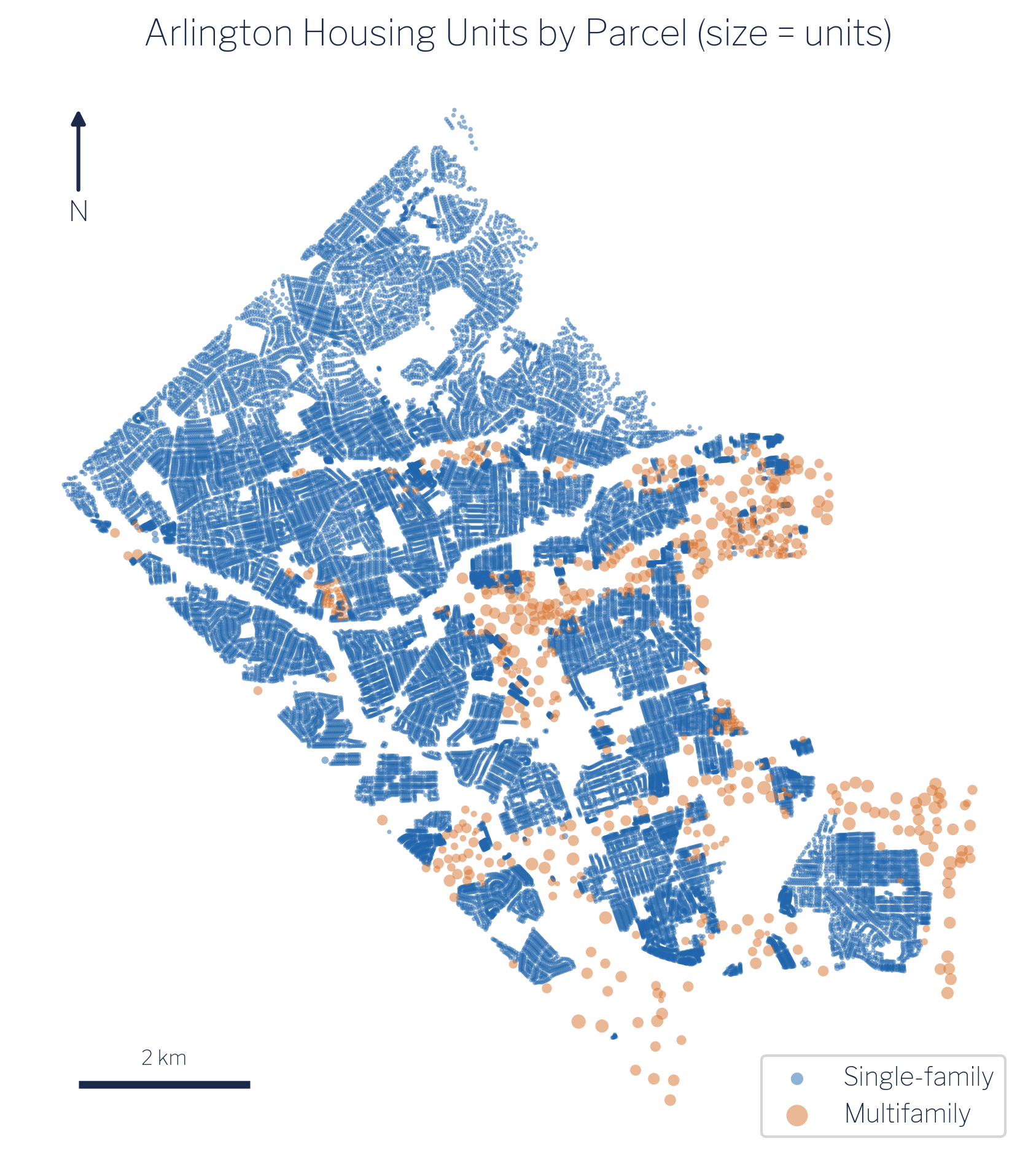
Figure 7.1 makes the spatial concentration vivid. A small number of large dots, each representing a multifamily building, account for a large fraction of the county’s residential footprint. The single-family parcels are numerous but individually small, spread across the county’s lower-density northern and western neighbourhoods. This heterogeneity is precisely what dasymetric redistribution is designed to exploit: instead of spreading a block group’s household counts uniformly across its entire polygon, we concentrate them where the housing units are.
7.2 The method: unit-weighted redistribution
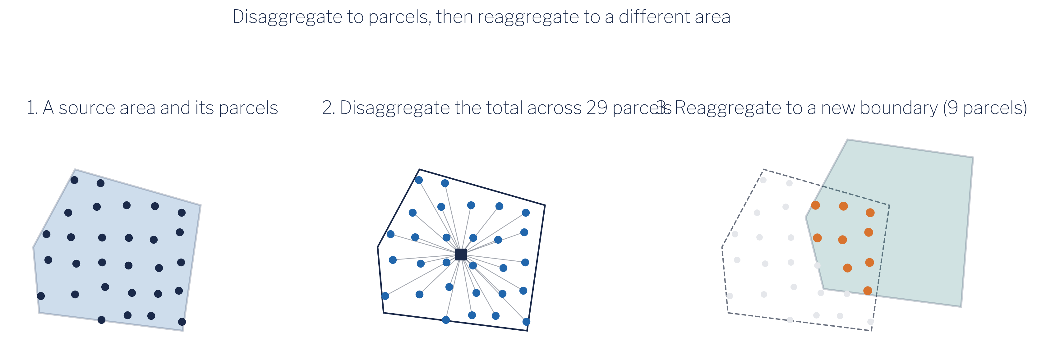
The implementation follows a straightforward unit-weighting scheme. Each parcel is “exploded” into a number of identical point records equal to its Total_Units count: a 300-unit multifamily building contributes 300 identical centroid points, while a single-family parcel contributes one. That pool of unit points is then passed to redistribute_parcels from the sdc-redistribute package, which uses the point locations as the dasymetric control layer. The block-group aggregate income and household counts are redistributed to civic associations in proportion to the number of unit points that fall within each association, weighted by their source block-group membership.
Figure 7.2 shows the spatial logic. A source block group’s total is divided across the parcels inside it, and those parcels are then collected under whatever target boundary we care about, here a civic association that overlaps the block group only partially. Only the parcels falling inside the target contribute to its estimate.
from sdc_redistribute import redistribute_parcels
# explode each parcel into Total_Units identical points first, then:
result = redistribute_parcels(
    source_df=counts_long, parcel_centroids=unit_points,
    source_geo="block_groups.geojson",
    target_geos={"civic_association": "civic_assoc.geojson"},
    count_cols=["agg_income", "households"], source_id="geoid",
)library(sf); library(sdc.redistribute)
# Split each block group's counts across its parcels, weighted by unit count.
civic <- redistribute_parcels(block_groups, civic, parcels,
extensive = c("agg_income", "households"),
weights = "Total_Units")
civic$mean_income <- civic$agg_income / civic$householdsThe logic is the same as the area-weighted approach (redistribute extensive counts, derive intensive rates afterward), with one structural difference: the implicit population surface has changed from a uniform density within each block group to a density proportional to the spatial distribution of housing units within that block group.
7.3 Results: a close agreement with the area-weighted estimates
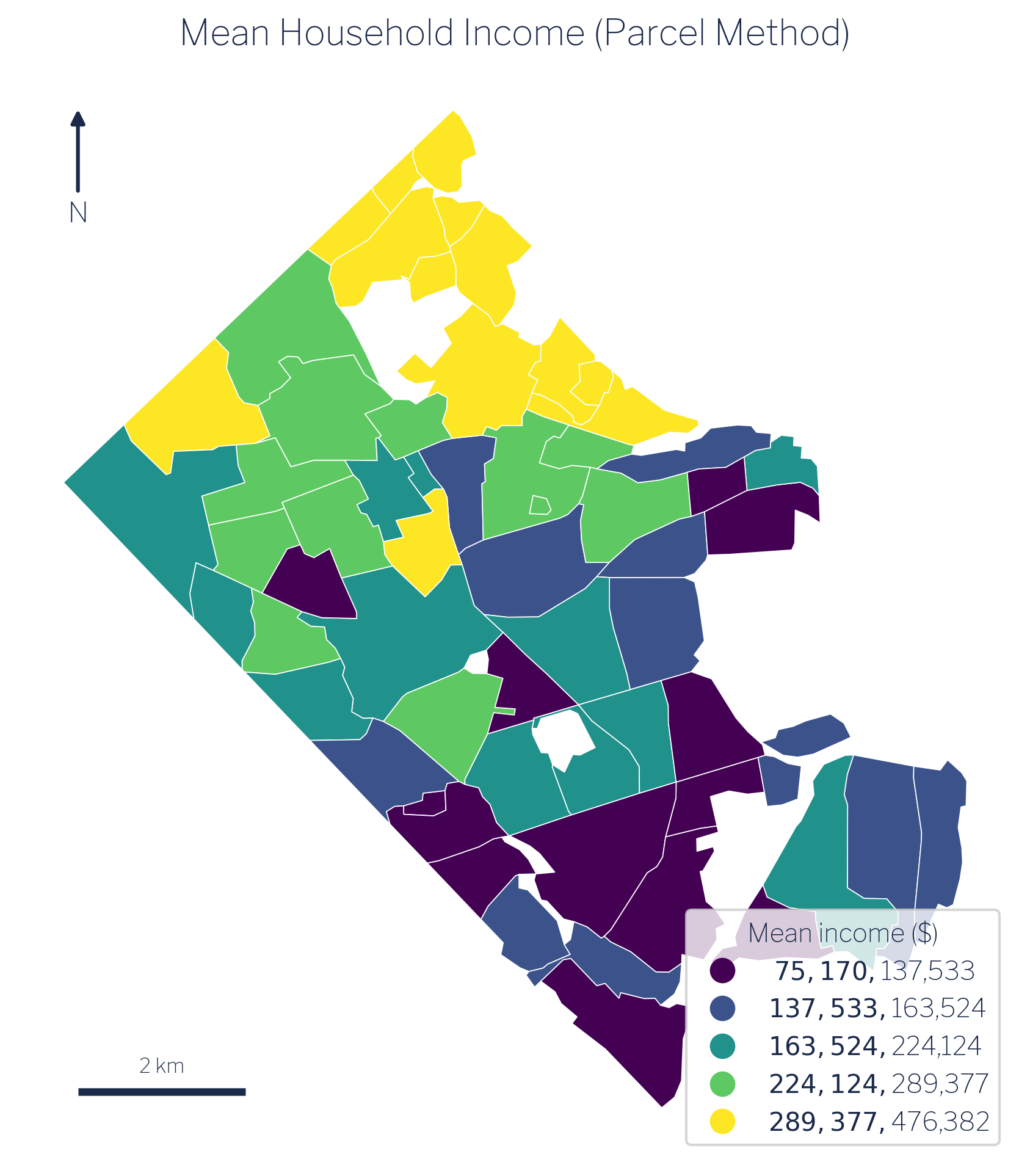
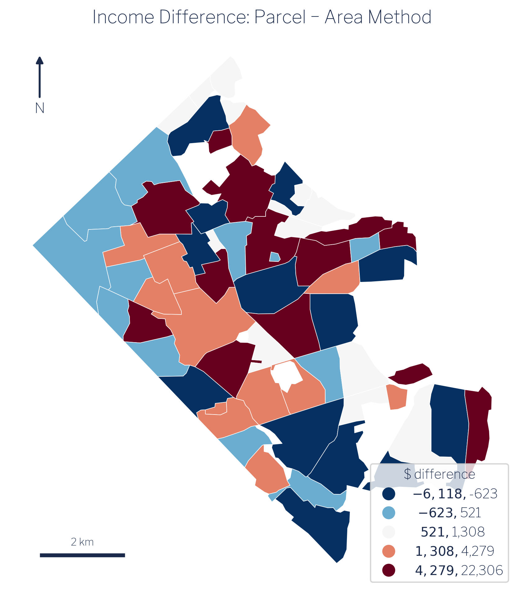
Figure 7.3 and Figure 7.4 tell a consistent story. The parcel map looks nearly identical to its area-weighted counterpart, and the difference map is dominated by values close to zero.
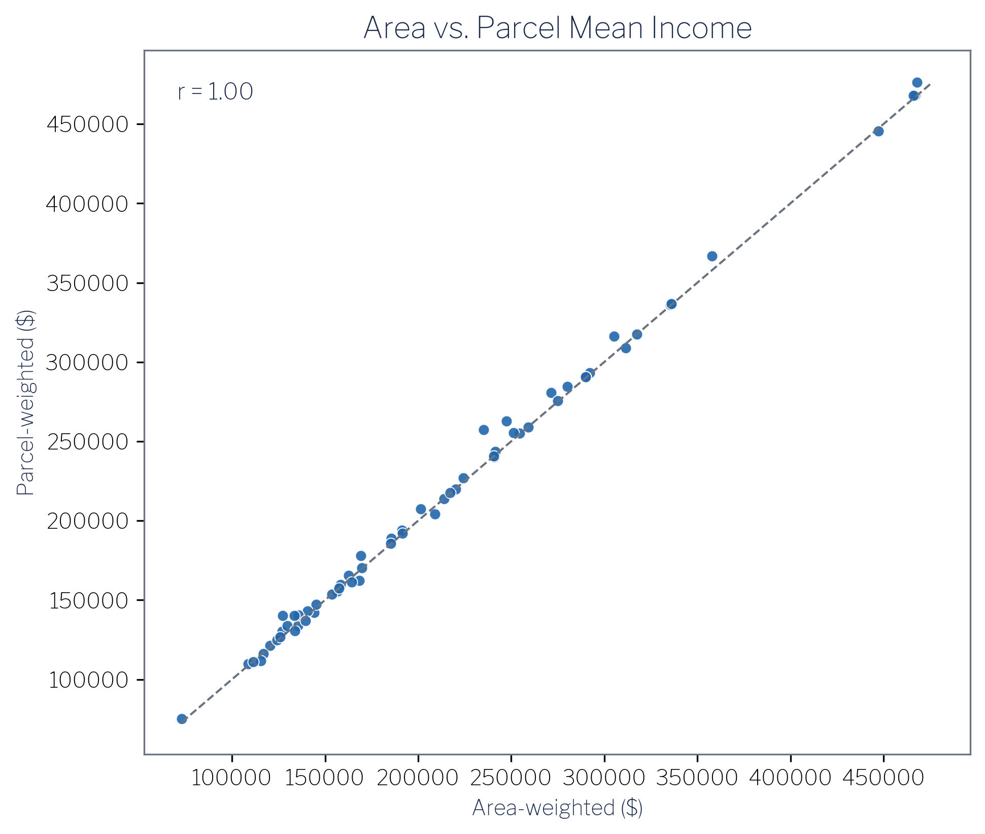
The scatter plot in Figure 7.5 makes the relationship explicit: the two methods produce a Pearson r = 1.00 across the 62 associations. The largest per-association shift in either direction is approximately ±$22,000, a few percent on six-figure incomes. The three biggest gainers under parcel weighting are Arlington Forest (+$22,306), Cherrydale (+$15,347), and Foxcroft Heights (+$13,047). The three biggest losers are Lyon Park (−$6,118), John M Langston (−$4,960), and Douglas Park (−$3,781).
Why do the methods agree so closely? Mean household income is a smooth, intensive measure: it describes a characteristic of households, not a count of things that accumulate over area. When a block group’s income is fairly evenly distributed among its housing stock, as it generally is in Arlington at the block-group scale, then where within the block group the housing sits barely changes the weighted average that reaches each civic association. Parcel placement shifts modest fractions of the income count from one association to an adjacent one, but because the income levels on both sides of any given boundary are similar, the effect on the mean nearly cancels. The ±$22,000 maximum shift represents the cases where a multifamily building with an unusually different household composition sits near a boundary: a real effect, but a small one relative to the income range in the data.
7.4 Leakage and the case for parcel weighting on count measures
One honest limitation deserves direct statement. Approximately 3,032 households (about 2.8% of the county total) sit in parcels whose centroids fall outside any civic association boundary. These households contribute to the block-group totals but are not allocated to any association under the parcel method. The parcel approach therefore slightly underestimates total households compared with the area-weighted method, which allocates every square metre of a block group to some association. Analysts using this method for official estimates should be aware of this leakage and decide whether to redistribute orphaned parcels to the nearest association or treat them as a separate “unassigned” category.
For mean income, which is what this guide measures, the 2.8% household leakage has a negligible effect on the ratio. For count measures (total population, total housing units), the answer is different. Dasymetric and parcel-based redistribution earn their keep precisely when the placement of housing within a block group drives the allocation of counts across target boundaries. If you want to know how many housing units fall within a specific civic association’s polygon, point-in-polygon counting on the parcel layer is more accurate than area weighting; the difference can be substantial in associations with compact boundaries or with multifamily buildings near their edges.
The natural next step in this direction is household-size weighting: single-family and multifamily units have systematically different average household sizes, and a redistribution that treats all units as interchangeable conflates these. The sdc-redistribute package’s redistribute_parcel_pums_adj function implements this extension by drawing on Public Use Microdata Sample (PUMS) household-size distributions, stratified by unit type, to weight single-family parcels differently from multifamily ones. Applying that method to Arlington’s MHUD data, and assessing whether the household-size correction changes the civic-association estimates meaningfully, is a planned extension of this work.
For the income analysis in this guide, the two methods are interchangeable in practice. The parcel approach is presented here to establish the infrastructure and to make a broader point: method choice matters most when the variable in question is a count and when housing is unevenly distributed within source units. When the variable is a smooth intensive measure like mean income, and when the redistribution is operating at the block-group-to-neighbourhood scale, area weighting and parcel weighting converge.