1 The Sub-County Data Gap
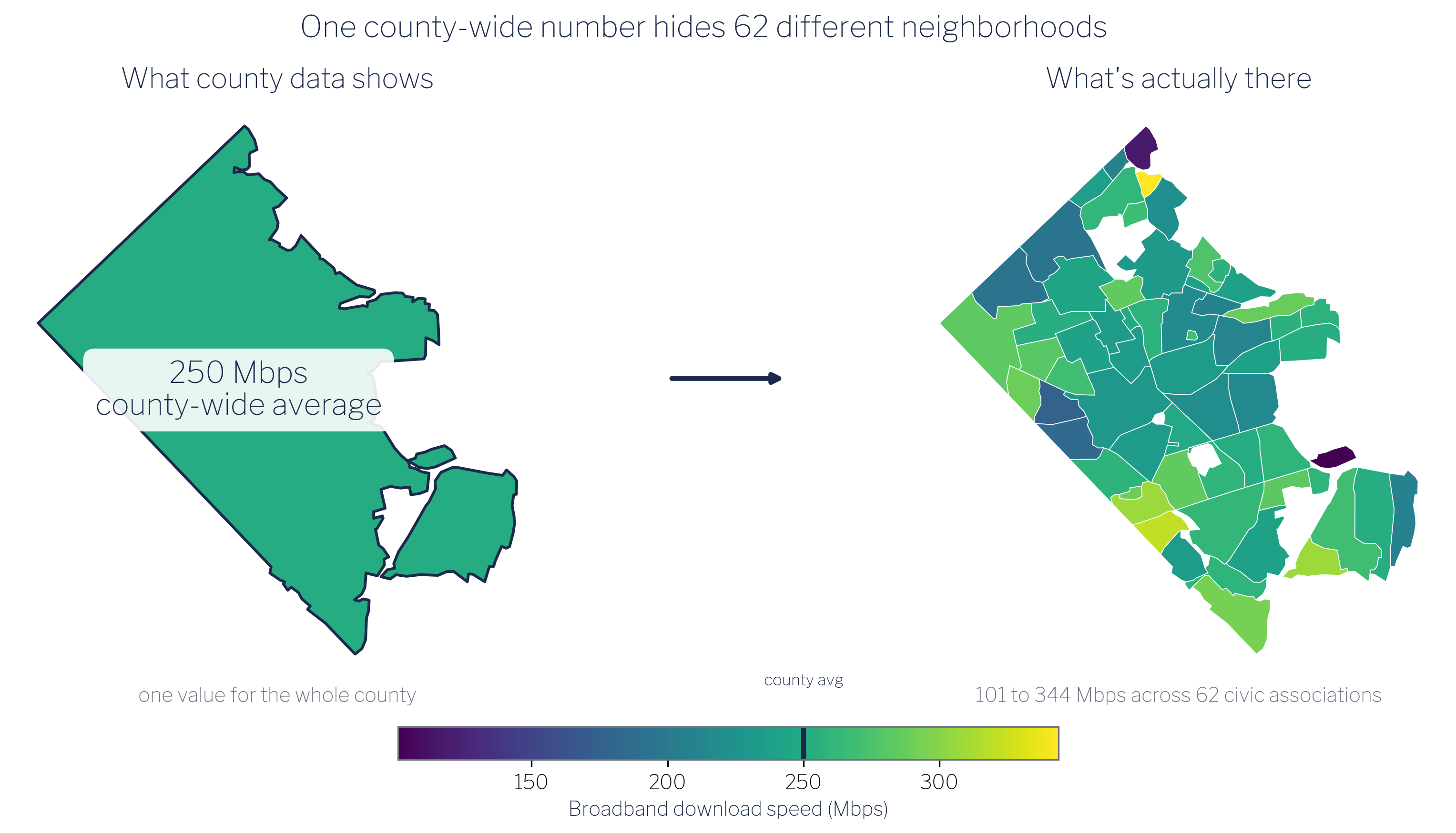
Local officials make decisions at the neighborhood level, but the data they rely on is usually reported at the county level. A county-wide broadband adoption rate, a county-wide income figure, a county-wide health outcome: these statistics obscure the variation that actually matters for policy. A neighborhood with near-universal high-speed service and an adjacent neighborhood with almost none look identical in a county aggregate. The officials who need to target investment, design interventions, or justify budget requests are working blind.
The units that drive real decisions are not counties. They are neighborhood associations, service districts, planning corridors, school catchment zones, and utility territories. These are the geographies where residents organize, where services are delivered, and where disparities become visible. County-level data cannot answer the questions local officials are actually asking.
1.1 Why sub-county data is scarce
The scarcity of reliable sub-county data has three overlapping causes. First, small-area estimates carry large statistical uncertainty: when a sample is divided into dozens of small geographic units, the counts per unit shrink, and margins of error grow until estimates become unreliable [1]. Second, statistical agencies and data providers apply geographic suppression or aggregation to protect individual confidentiality; the smaller the area, the more likely a cell will be suppressed [2]. Third, there is no standardized collection infrastructure at the sub-county level. Unlike counties or census tracts, neighborhood and civic-association boundaries are locally defined, vary across jurisdictions, and change over time, so no national data program routinely publishes estimates for them [3].
The result is a persistent data gap between the geographic scale at which data is collected and reported and the geographic scale at which local government operates. Analysts working inside local government (and researchers trying to support them) must construct the sub-county datasets they need rather than retrieve them from a shelf [4].
1.2 What this guide demonstrates
This guide works through a concrete example: estimating mean household income and fixed-broadband download speeds for each of Arlington County, Virginia’s 62 civic associations, which together cover approximately 109,528 households. The two source datasets (Ookla fixed-broadband speed-test tiles and American Community Survey block-group income and household counts) arrive on entirely different geographic footprints that match neither each other nor the civic-association boundaries. The guide shows, step by step, how to align those footprints through areal-weighted interpolation and produce estimates at the policy-relevant geography.
The worked example is implemented in both Python and R. The two produce the same estimates; each stage later in the guide shows the code in both languages, and the complete source for each is in the code appendices.
Local government analysts will find a reproducible workflow they can adapt to their own jurisdiction, data sources, and policy geographies. The method generalizes beyond broadband and income to any pair of spatially misaligned datasets.
Decision-makers and program managers can read the prose and figures without engaging the code. The key takeaways are in the chapter narratives and maps. The technical sections are clearly marked.
Some background in geographic data is helpful but not required. The guide explains each concept as it arises.